t.b.d.

Our implementation of label/2 does a backtracking search strictly from left to right. One can easily verify that reordering the variable order doesn't change the result. The same number of solutions should be always returned. On the other hand reordering can drastically change the workload and thus the time spent in searching for solutions.

Some constraint solvers try to break out of the given variable order by forms of forward checking. The idea is simply if a present instantiated constraint can be logically reduced to X = C, where X is another attribute variable and C is a constant, I can trigger a new bind/2 call. We do not provide forward checking in indomain/2.

Instead we adress what was already at the heart of the Wong & Youssefi query plan generator for the INGRES database. Namely we reorder the variables based on a scoring. While Wong & Youssefi used cardinality, we can consider the number of k of free variables in a constraint. For a domain |D| = n, this leads in the maximum to a cardinality n^k, so that our score is the logarithm of the cardinality.

/* The predicate succeeds with the number of free variables. */
score('$ATTR'(V,L), P, S) :- var(V), !,
   term_variables(P+L, H),
   length(H, S).
score(_, _, 0).

While Wong & Youssefi observe that with a score and further estimates such as success rates, the problem can turn into a dynamic programming problem. We follow Wong & Youssefi in that we apply a greedy heuristic and simply pick a variable with the lowest score. Doing this repeatedly and statically, and even tracking the variable history, we get an ahead of time computation of a variable order based on an abstract score:

/* The predicate succeeds with the heuristically reordered variable order. */
ahead([], _, []).
ahead([X|L], P, [Y|R]) :-
   score(X, P, S),
   best(L, P, S, 1, 0, I),
   nth0(I, [X|L], Y, H),
   deref(Y, Z),
   ahead(H, [Z|P], R).

SWI-Prolog does the same when using its ff strategy, only it does so dynamically during labeling. It also uses a more concrete score than we do, based on the actual reduced domain. This means different constraint solving states can lead to different variable orderings, so that not all solutions are the result of the same variable order. While in our approach the variable order is only determined once ahead of time:

/* The predicate binds the elements of L, heuristically reordered. */
labeling(L, D) :-
   ahead(L, [], R),
   label(R, D).

Since the library(edge/railgun) provides the set of predicates for modelling and solving constraint problems, that has become a defacto standard among a couple of Prolog systems, it becomes relatively easy to run existing models. There are only a few precautions necessary, for example term_variables/2 should be called before the model is built, otherwise it will only see the value holders and not the attributed variables.

As an example we take the Sudoku modelling, as published on the website of SWI-Prolog. It demonstrate that it can be modelled as is with our Lean CLP library(edge/railgun). To do that we first need a little helper, namely the transpose of a matrice. Matrices are used in the modelling to represent a Sudoku board. We take some code by Carlo Capelli, published on stackoverflow in December 7, 2015:

transpose([], []).
transpose([U], B) :- !, sys_gen(U, B).
transpose([H|T], R) :- transpose(T, TC), sys_splash(H, TC, R).

sys_gen([], []).
sys_gen([H|T], [[H]|RT]) :- sys_gen(T,RT).

sys_splash([], [], []).
sys_splash([H|T], [R|K], [[H|R]|U]) :- sys_splash(T,K,U).

?- transpose([[1,2],[3,4]], X).

The predicate sudoku/1 constrains a partially instantiated board:

:- ensure_loaded(library(edge/railgun)).

sudoku(M) :-
   maplist(all_different, M),
   transpose(M, H),
   maplist(all_different, H),
   groups(M).

groups([]).
groups([As,Bs,Cs|L]) :- blocks(As, Bs, Cs), groups(L).

blocks([], [], []).
blocks([N1,N2,N3|Ns1], [N4,N5,N6|Ns2], [N7,N8,N9|Ns3]) :-
   all_different([N1,N2,N3,N4,N5,N6,N7,N8,N9]),
   blocks(Ns1, Ns2, Ns3).

In the above we differ from the website of SWI-Prolog, in that we use the weaker all_different/1 constraint and not the stronger all_distinct/1 constraint. The stronger predicate is not available in our Lean CLP since we have banned forward checking. In certain circumstances the stronger all_distinct/1 is powerful enough to solve a problem without labeling. To solve Markus Triskas example given on the website of SWI-Prolog, we have to use labeling:

problem(8, [[_,_,_,_,_,_,_,_,_],
            [_,_,_,_,_,3,_,8,5],
            [_,_,1,_,2,_,_,_,_],
            [_,_,_,5,_,7,_,_,_],
            [_,_,4,_,_,_,1,_,_],
            [_,9,_,_,_,_,_,_,_],
            [5,_,_,_,_,_,_,7,3],
            [_,_,2,_,1,_,_,_,_],
            [_,_,_,_,4,_,_,_,9]]).

?- problem(8, _M),
   term_variables(_M, _L),
   sudoku(_M),
   time(once(labeling(_L, [1,2,3,4,5,6,7,8,9]))),
   maplist(maplist(deref), _M, R).

Markus Triskas problem #8 is among the harder Sudoku problems. Nevertheless Lean CLP can produce a first solution in about 5 seconds on a modern AI laptop, using our ahead of time variable ordering predicate labeling/2. We tested with an AMD Ryzen 7 350 CPU which was released to the public in Januar 2025. We were also currious how this compares to other Prolog systems.

We used a couple of Sudoku problems of varying difficulty:

#1: 050009000176500380003060500000700000095030270
    000004000002090100031008945000100030
#2: 000605009410000020000000107000938600004000200
    709000000000183000060020030028000050
#3: 090000400008500010001000068000100030000045700
    050007000070090200003600000800000000
#4: 845060003700109400000080006002000045000000000
    530000100200030000001905008300020754
#5: 000037000020100000900200850056000001010604090
    200000380065003004000005070000900000
#6: 000036040017000000000080070040000000305000900
    000107002004000000720000009850002400
#7: 000806000050100000300400200001090000008000300
    000050407020000000400000000000000010
#8: 000040009002010000500000073090000000004000100
    000507000001020000000003085000000000

Among the tested Prolog systems were SWI-Prolog 9.3.35 and Trealla Prolog 2.86.3 again. The testing was carried out outside of the browser using the Windows 11 command line and precompiled .exe binaries. In as far we tested against Dogelog Player 2.1.4 for the Java target, and not for the JavaScript target. To be comparable with our modelling and search, we kept the all_different/1 modelling and used the labeling/2 predicate of the Prolog systems, with the fail fast (ff) option.

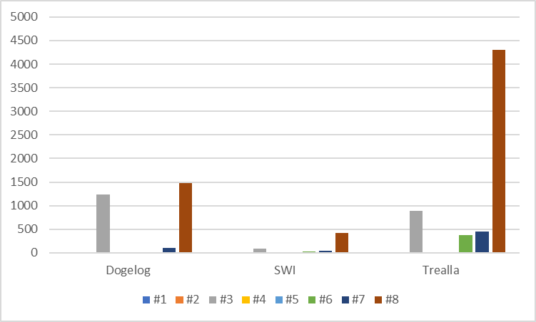
The test results show, that as expected the fail fast (ff) option of SWI-Prolog fares better. For reasons that ff is the dynamic and concrete variant of a our heuristic reordering, it gives better results. On the other hand Trealla lacks behind, has probably to do that it already lacks behind in the under constrainted permutation and map coloring problems. Trealla makes problem #6 and #7 look harder than for the other Prolog systems.

The benchmark profile is sparky, and one can experiment with permuted problems and one will see that the spikes change their pattern. The labeling/2 predicate in Lean CLP and also in the other Prolog systems is still sensitive to the input order, since the heuristic reordering has to make decisions among variables that show a tie in their scoring. Despite the small sample set, if we sum the runtimes we get 2860ms Dogelog, 597ms SWI-Prolog and 6061ms Trealla, which puts our Lean CLP in the midfield.

Since the recent version of Dogelog Player supports cyclic terms, we could let the Jini out of the bottle, and provide the experimental library(edge/railgun) to model delayed goals with nothing else than the ISO core standard Prolog and Alain Colmerauers rational trees. The result is a Lean CLP of ca. 100 lines of code, that already provides a simple constraint (#\=)/2 and a global constraint all_different/1.

The results are encouraging. For problems that are not over constrained, Dogelog Player leaves existing Prolog systems clearly behind, showing a 2-3x times speed-up against SWI-Prolog and a 20-30x times speed-up against Trealla Prolog. For more constrained problems we suggest ommiting forward checking in favor of a form of ahead of time (AOT) variable ordering. With this approach and for Sudoku problems we are then in the midfield between SWI-Prolog and Trealla Prolog.